Intro of Basic Machine Learning Concepts

Basic Machine Learning Concepts

This MD file is to test the LaTeX display

1. Overfitting / Underfitting

   • Overfitting refers to a model that matches the training data too closely, including its noise and outliers, which diminishes the model’s ability to generalize to new data. This results in excellent performance on the training set but poor performance on validation/test sets.

     • Solutions to overfitting generally include:
     1. Reducing the number of features appropriately.
     2. Adding a regularization term. Regularization aims to reduce the influence of features on the prediction outcome. Common regularization terms include L1 and L2 regularization.

   • Underfitting is the opposite, where the model lacks sufficient complexity to capture the underlying patterns in the data.

     • Solutions to underfitting include:
     1. Increasing the number of training epochs.
     2. Adding more features to the model.
     3. Reducing the regularization term.

2. Bias / Variance Trade-off

   • Bias refers to the difference between the model’s predicted values and the actual values, describing the model’s fitting ability.
   • Variance describes the model’s sensitivity to different datasets, indicating how much the data fluctuations affect the model.

   Generally, simpler models have higher bias and lower variance, while more complex models have lower bias and higher variance. This also corresponds to the concepts of overfitting and underfitting.

   A common method to balance bias and variance is cross-validation. The basic method of k-fold cross-validation is to divide the training set into k parts. Each time, one part is used as the validation set, and the remaining k-1 parts are used as the training set. This process is repeated k times, ensuring that each part is used as the validation set. The final loss is the average of the k training losses.

Regularization

1. L1 vs. L2 Regularization

   • L1 Regularization, also known as LASSO, is the sum of the absolute values of all parameters.

     $$\| x \|_1 = \sum_{i=1}^{m} |x_i|$$

   • L2 Regularization, also known as Ridge, is the square root of the sum of the squares of all parameters.

     $$\| x \|_2 = \sqrt{\sum_{i=1}^{m} x_i^2}$$

   • Both types of norms help reduce the risk of overfitting. L1 norm can be used for feature selection, but it cannot be directly differentiated, so conventional gradient descent/Newton’s method cannot be used for optimization. Common methods include coordinate descent and Lasso regression. L2 norm is easier to differentiate.

2. Sparsity of L1 Norm / Why L1 Regularization Can Be Used for Feature Selection

   Compared to L2 norm, L1 norm is more likely to yield sparse solutions, meaning it can optimize unimportant feature parameters to 0.

• Understanding this:

  Suppose the loss function $L$ has a certain relationship with a parameter $x$ as shown below. The optimal point is at the red dot where $x < 0$.

  • Adding L2 regularization results in a new loss function $L + Cx^2$, where the optimal $x$ is at the blue dot, reducing $x$’s absolute value but still non-zero.

  • Adding L1 regularization results in a new loss function $L + C|x|$, making the optimal $x$ equal to 0.

  When L2 regularization is added, the loss function’s minimum at $x = 0$ occurs only when the original loss function’s derivative is zero. With L1 regularization, $x = 0$ becomes a minimum point if the parameter $C$ and the loss function’s derivative satisfy $C > |L|$.

  L1 regularization leads to many parameters becoming zero, making the model sparse, which can help in feature selection.

Evaluation Metrics in Machine Learning

1. Precision / Recall / F1 Score

   For binary classification problems, precision, recall, and F1 score are often used to evaluate the model’s performance. The prediction results can be divided into:

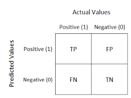
   • TP (True Positive): Correctly predicted positive class.
   • TN (True Negative): Correctly predicted negative class.
   • FP (False Positive): Incorrectly predicted positive class.
   • FN (False Negative): Incorrectly predicted negative class.

   Definitions:

   • Precision: The ratio of correctly predicted positive observations to the total predicted positives.

     $$P = \frac{TP}{TP + FP}$$

   • Recall: The ratio of correctly predicted positive observations to all observations in the actual class.

     $$R = \frac{TP}{TP + FN}$$

   • F1 Score: The harmonic mean of precision and recall.

     $$F_1 = \frac{2 \times P \times R}{P + R} = \frac{2TP}{2TP + FP + FN}$$

2. Confusion Matrix

   The confusion matrix for classification results is shown below:

   

3. Macro-F1 vs. Micro-F1

   When there are multiple binary classification confusion matrices (e.g., multiple training and testing datasets/multiple datasets/pairwise combinations in multi-class tasks), we want to evaluate the model performance comprehensively across n binary classification confusion matrices.

   • Macro-F1: Directly calculate the precision and recall for each confusion matrix, then average them to get macro-P, macro-R, and the corresponding macro-F1.

     $$\text{macro-}P = \frac{1}{n} \sum_{i=1}^{n} P_i, \qquad \text{macro-}R = \frac{1}{n}\sum_{i=1}^n R_i,$$
     $$\text{macro-}F_1 = \frac{2 \times \text{macro-}P \times \text{macro-}R}{\text{macro-}P + \text{macro-}R}$$

   • Micro-F1

     Another approach is to first average the corresponding elements of each confusion matrix to obtain $\overline{TP}$, $\overline{TN}$, $\overline{FP}$, and $\overline{FN}$. Then, based on these values, calculate micro-$P$, micro-$R$, and the corresponding micro-$F_1$.

     $$\text{micro-}P = \frac{\overline{TP}}{\overline{TP}+\overline{FP}}, \qquad \text{micro-}R = \frac{\overline{TP}}{\overline{TP}+\overline{FN}},$$
     $$\text{micro-}F_1 = \frac{2 \times \text{micro-}P \times \text{micro-}R}{\text{micro-}P + \text{micro-}R}$$

4. ROC Curve / AUC Area

   ROC Curve (Receiver Operating Characteristic) and AUC (Area Under ROC Curve) are the most commonly used evaluation metrics for imbalanced classification problems. To understand what ROC is, we first define two metrics based on the confusion matrix: True Positive Rate (TPR) and False Positive Rate (FPR).

   $$TPR = R = \frac{TP}{TP+FN}, \qquad FPR = \frac{FP}{TN+FP},$$

Ideally, a good model should satisfy high TPR and low FPR. For any trained model, we can calculate its TPR and FPR on the given test data. By plotting FPR on the x-axis and TPR on the y-axis, we can represent any model’s (FPR, TPR) pair in this coordinate system, as shown in the figure below. The space constructed by this coordinate system is called the ROC space. In the example, there are five models: A, B, C, D, and E. In the ROC space, the closer a model is to the top left corner, the better it is.

In most binary classification problems (especially in neural networks), the decision to classify a sample as positive or negative is based on setting a threshold. If the value exceeds this threshold, the sample is labeled as positive; otherwise, it is labeled as negative. Usually, this threshold is set to 0.5. If we try different thresholds to separate positive and negative classes, we can obtain multiple (FPR, TPR) pairs. By plotting these pairs, we can draw a curve in the ROC space, known as the ROC Curve. If the (FPR, TPR) points are sufficiently dense, we can calculate the area under the curve, known as the AUC Area.

Loss and Optimization

1. Convex Optimization Problems

   An optimization problem is a convex optimization problem if its objective function is a convex function and the feasible region is a convex set (a set where any line segment between two points in the set lies entirely within the set).

   A function $f$ defined on a convex domain $\mathbb{D}$ is convex if and only if for any $x, y \in \mathbb{D}$ and $\theta \in [0, 1]$, we have:

   $$f(\theta x+(1-\theta)y) \le \theta f(x)+(1-\theta) f(y)$$

The importance of convex optimization problems in mathematics lies in the fact that the local optimum of a convex optimization problem is also its global optimum. This property allows us to use greedy algorithms, gradient descent methods, Newton’s methods, etc., to solve convex optimization problems. In fact, many non-convex optimization problems are solved by breaking them down into several convex optimization problems and solving them individually.

2. MSE / MSELoss

   Mean Square Error (MSE) is the most common metric in regression tasks.

   $$E(f;D)=\sum_{i=1}^m (f(x_i) - y_i)^2$$

3. Is Logistic Regression with MSELoss a Convex Optimization Problem?

   No. Logistic regression maps a linear model to a classification problem through the sigmoid nonlinear function. Its MSE is a non-convex function, and the optimization process might result in a local optimum instead of a global optimum. Therefore, logistic regression with MSELoss is not a convex optimization problem.

4. Relationship Between Linear Regression, Least Squares Method, and Maximum Likelihood Estimation

   The common methods for solving linear regression are the Ordinary Least Squares (OLS) method and the Maximum Likelihood Estimation (MLE) method.

   • The least squares method uses the sum of the squared differences between predicted and actual values as the loss function (MSELoss).

     $$J(w)=\sum_{i=1}^m (h_w(x_i) - y_i)^2$$

   • Maximum likelihood estimation estimates the model parameters $h_w$ by maximizing the likelihood of the observed data. Given $x$ and $y$, it estimates the most likely model parameters. Assuming the error $\epsilon_i = y_i - h_w(x_i)$ follows a Gaussian distribution, the probability density function is:

     $$p(\epsilon_i) = \frac{1}{\sigma \sqrt{2\pi}} e^{-\frac{(\epsilon_i)^2}{2\sigma^2}}$$

     Substituting $\epsilon_i = y_i - h_w(x_i)$, we get:

     $$p(y_i | h_w(x_i)) = \frac{1}{\sigma \sqrt{2\pi}} e^{-\frac{(y_i - h_w(x_i))^2}{2\sigma^2}}$$

     The likelihood function is:

     $$L(h_w(x_i)) = \prod_{i=1}^m p(y_i | h_w(x_i))$$